|
|
|
 |
General
The objective of FIR filters adaptation is to (asymptotically) bring
the values of one FIR filter coefficients (the adapting filter) to the
values of another FIR filter coefficients (the reference filter). The
adaptation mechanism is based on comparing the way the adapting filter
responds to an input stimulus with the way the reference filter
responds to the same stimulus, and changing the adapting filter's
coefficients so that its response resembles (as closely as possible)
the response of the reference filter (Fig.10).
The adaptation mechanisms depend on the type of filter that is being
adapted, and on various characteristics of the input stimuli, i.e. it
is not the same mathematical model that is used for all types of
filters. This section describes an adaptation method used for FIR
filters when the input stimulus is a random signal.
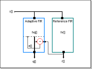
Fig.10: Adaptive FIR Block Diagram
The Adaptation Mechanism
Using the notations in Fig.10 (x[] is the input signal, q[] is the adapting filter's output, r[] is the reference filter's output, and e[] is the output error), and the results presented in the FIR filters section, the following set of formulae can be derived for the elements of the q[], r[], and e[] vectors:
r[n]=Sum(hr[k] x[n-k]), k in [-N/2, N/2-1]; where hr[] is
the reference filter's weights vector
q[n]=Sum(hq[k] x[n-k]), k in [-N/2, N/2-1]; where hq[] is
the adapting filter's weights vector
e[n]=r[n]-q[n]
The adaptation process will have to result in matching (as close as
possible) the values of hq[] with hr[]. As a measure of the adaptation
status, the distance between hr[] and hq[] (seen as vectors in an
N-dimensional vector space) will be considered; adapting hq[] to hr[]
will thus be equivalent to minimizing this distance.
The Weights Error Function will now be introduced:
Eh(n) = 1/N Sum((hr[k](n)-hq[k](n))^2), k in [-N/2, N/2-1];
here Eh(n) is the weights error function calculated at moment n, based
on the hr[](n) and hq[](n) vectors' components at moment n.
However, the only available data about the adapting FIR internal
status is its response to the input signal; thus, in order to match the
q[n] response with r[n], an attempt will be made to minimize the output
error e[].
A Response Error Function E() will now be introduced:
E(n) = 1/M Sum(e[n-m]^2), m in [0, M-1]; here E(n) is the
response error function calculated at moment n, based on the e[] error
vector's last M values.
By minimizing the sum of squares E(n), each of last individual error
values (i.e. e[m] with m in [n, n-M+1]) will also be minimized. Since
the e[m] components are the output error values q[m]- r[m], the last M
difference values (q[m] - r[m] with m in [n, n-M+1]) will be minimized.
The goal:
e[n] = 0
implies:
Sum( (hq[k]-hr[k])x[n-k] ) = 0, k in [-N/2, N/2-1];
The above formula can be seen as a filtering operation of an impulse
hq[]-hr[] with a filter having the frequency-domain characteristic
FT(x[]) (see also the FFT/iFFT section).
If FT(x[]) is non-null in the entire FT domain, the above condition
results in having hq[]-hr[] = 0, i.e. hq[k]=hr[k] with k in [-N/2,
N/2-1] (see the Remark at the end of this section).
The adaptation process will consist of updating each component h[k]
along the gradient of the response error function (on the corresponding
direction), at each moment n:
h[k](n+1) = h[k](n) - beta d(E)/d(h[k])(n); here beta is a
factor that controls the adaptation speed.
Calculations result in the following Reference Formula:
h[k](n+1) = h[k](n) + beta 2/M Sum(e[n-m] x[n-m-k]), m in
[0, M-1]
Two commonly used algorithms have been derived from the above formula:
- the Least Mean Square (LMS) algorithm is obtained by setting M=1:
h[k](n+1) = h[k](n) + 2 beta e[n] x[n-k] - the Bloc-update algorithm is obtained when only a part of the
coefficients are updated at each new sample, so that all the
coefficients get updated only once every M samples:
h[k](n+1+M) = h[k](n) + 2 beta e[n+M] x[n-k+M]
Remark
All the above line of thinking is based on having FT(x[]) non-null in
the entire FT domain; highly random input signals (with sharp
autocorrelation functions) have this property. However, there are
signals x[] for which the condition Sum((hq[k]-hr[k])x[n-k]) = 0 does
not imply hq[k]-hr[k]=0; a class of such signals are the periodic
signals (with few spectral components), for example sine waves (see
also the Correlation/Autocorrelation section).
This is exemplified in Fig.11: Fig.11a shows the coefficients of a
reference low-pass FIR filter, and Fig.11b, Fig.11c, Fig.11d, and
Fig.11e show the adaptation process of an FIR filter for the two types
of input signals:
Fig.11b shows the evolution of the adapting FIR filter coefficients'
when a sinewave input signal is being used; it can be seen that the
coefficients did not adapt correctly (this is possible because there
are many sets of FIR coefficients that produce the same output for a
sinewave input signal).
Fig.11c shows the evolution of the adapting FIR filter coefficients'
when a highly random input signal is being used; it can be seen that
the FIR coefficients adapt correctly to the values of the reference
filter (and consequently the FIR output will match the output of the
reference filter). Fig.11c - Zoom1 is a zoom on the initial phase of
the adaptation.
Fig.11d shows the response error function E() and weights error
function Eh() for a sinewave input; it can be seen that the weights
error function Eh() does not decrease although the response error
function E() decreases (i.e. the filter does not adapt).
Fig.11e shows the response error function E() and weights error
function Eh() for a highly random input; it can be seen that both the
weights error function Eh() and the response error function E()
decrease (i.e. the filter adapts).
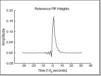 Fig.11a |
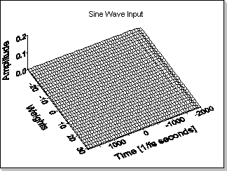 Fig.11b |
||
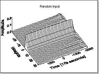 Fig.11c |
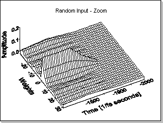 Fig.11c zoom |
||
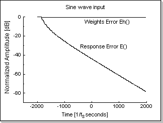 Fig.11d |
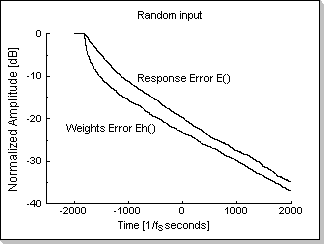 Fig.11e |
Adaptation Speed
In the LMS-update formula:
h[k](n+1) = h[k](n) + 2 beta e[n] x[n-k],
it can be seen that the h[k] increments (and thus the adaptation speed)
depend on beta, and on the magnitudes of e[] and x[].
Fig.12a shows the weights error function during the adaptation
process for two values of beta, using the same input signal; decreasing
beta by two results in decreasing the adaptation speed by two.
Fig.12b shows the weights error function during the adaptation process
using the same beta coefficient, but using two input signals;
decreasing input signal's amplitude by two results in decreasing the
adaptation speed by four.
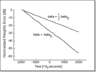 Fig.12a |
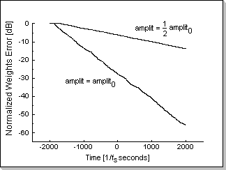 Fig.12b |
Note 1
The adaptation speed is reflected in the slope of the plots in Fig.12a
and Fig.12b
Note 2
In Fig.12a and Fig.12b a leaky integration -based short-time average of
the Weights Error Function Eh(n) has been chosen for representation
instead of the Eh(n) function itself, in order to smoothen the plotted
graphics:
Eh_plot(n) = plot_cst Eh(n) - (1 - plot_cst) Eh_plot(n-1);
where plot_cst is a factor controlling the averaging interval.
Dynamic Correction of the Adaptation Speed Factor
Since e[] is proportional with x[] it results that the overall speed of
adaptation is inverse proportional with the squared magnitude of x[],
i.e. the power of the input signal. A leaky integration -based measure
of the input signal's average power is now introduced:
W(n) = alpha x[n]^2 + (1-alpha) W(n-1)
In order to compensate the variation of the adaptation speed with the
power of the input signal, in most echo cancellers the constant
adaptation speed factor beta is replaced with a correction function
that is dependent on the average power of the input signal:
beta <=> beta/W(n)
Thus, the following adaptation formula results:
h[k](n+1) = h[k](n) + 2 beta/W(n) e[n] x[n-k]
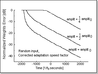
Fig.13
Fig.13 shows the adaptation process for three input signals using the corrected adaptation factor formula. Despite the three different amplitudes, it can be seen that the adaptation speeds (reflected in the slope of the three plots) rapidly converge to approximately the same value.
Conditions for the numeric values involved in the Adaptive FIR
calculations
The numeric conditions that were deduced in the FIR filters section
also apply to adaptive FIR filters; however, some other restrictions
may apply, depending on the specific adaptation algorithm.
For example, in the case of the LMS algorithm, the adaptation step must
be guarded against overflow:
2 beta e[n] x[n-k]
This condition will always hold true if:
2 beta x[n-k] < 1
Depending on the value of beta and the number of FIR taps, this
condition may be more restrictive than the FIR-inherited conditions
(however, this would only happen for very large values of beta that are
not used in practice).
Remark
Each specific adaptation algorithm (or variation of it) may require the
introduction of further restrictions in order to prevent internal
overflows; this problem has to be studied on a per-algorithm basis (the
LMS-based Echo Canceller is one such example where a number of
optimizing procedures imply new restrictions on the numeric values).
The Adaptive FIR Implementation (fig. 10)
The Adaptive FIR Components:The Adaptive FIR module has the following user-accessible interface elements:
- an input buffer vector x[] of P elements: it stores the input values that are necessary to compute the estimated adapting filter response
- an error input: via this variable the reference filter output is input in the adaptive filter
- the adapting weights buffer vector hq[]; it has the same number of elements as the input vector x[]
- a power-type specifier: this specifier selects between two ways of measuring the input signal's short-time average value, using either the signal's peak or mean level (this specifier defaults to peak)
- leak factor: used for computing the input's short-time mean or peak value with leak-based algorithms (this variable defaults to a pre-defined value)
- threshold: the weights buffer vector hq[] is updated only if the current input signal's average level (computed according to the power-type specifier) is above the threshold level (this variable defaults to a pre-defined value)
- beta: this controls the relative convergence speed, i.e. filter adaptation speed (this variable defaults to a pre-defined value)
- a function that defines the size P of the input buffer
- a function that pre-fills the whole input buffer vector x[]
- a function that introduces one input value at a time into the input buffer vector x[]
- a function that inputs the reference filter's current output into the adaptive filter's error input
- a function that updates all the values in the hq[] weights buffer vector; this function has two variants that are each optimized for non-causal and causal adaptive filters respectively
- a reset function that clears both the x[] and hq[] vectors, and marks P as unassigned (set to -1)
The function that updates the hq[] weights buffer vector implements an updating formula that is different from the LMS Reference Formula.
The LMS Reference Formula:
h[k](n+1) = h[k](n) + 2 beta e[n] x[n-k]
is being replaced by the following formula:
h[k](n+1) = h[k](n) + 2 beta e[n-1] x[n-k-1]
This approach is taken to take advantage of the hardware resources specially designed into the CDSP family.
It can be seen that the modified formula differs from the Reference Formula by updating the weights one sample later. The convergence performance and all other characteristics remain unchanged when using the modified formula.
The Adaptive FIR usage:
For the general non-causal Adaptive FIR: given the fact that the computation of the adaptive filter response to an input requires P input values to be known (i.e. x[n-P/2+1] to x[n+P/2]), it results that the first update of the weights buffer vector hq[] can only be done after introducing P input samples in the adaptive filter (this can be done via P successive calls to the function that introduces one input sample at a time into the input buffer vector x[]). These samples will represent P/2-1 samples "from the past", the "present" sample, and P/2 samples "from the future" in a time-domain interpretation (non-causal filters adaptation requires samples from both "before" and "after" the "present" moment). After introducing these P samples and the current response of the reference filter to the inputs of the adaptive filter, one will be able to update the hq[] weights by calling the hq[] update function for the first time. A new hq[] update can further be calculated after each introduction of a new pair of {input sample, reference filter response}. Thus, the methodology of adapting a Non-Causal FIR filter will consist of:
- introducing P/2-1 samples "from the past" (x[n0-P/2+1] to x[n0-1])
- introducing the "present" sample (x[n0])
- introducing P/2 samples "from the future" (x[n0+1] to x[n0+P/2])
- introducing the reference filter's response
- updating the hq[] weights buffer vector for the first time by calling the hq[] update function
- repetitively introducing new pairs of {input sample, reference filter response} representing input values "from the future" taken at time "present"+P/2 {x[n+P/2], r[n+P/2]}, and updating the hq[] weights
- introducing P/2-1 samples "from the past" (x[n0-P/2+1] to x[n0-1])
- introducing the "present" sample (x[n0])
- introducing the reference filter's response
- updating the hq[] weights buffer vector for the first time by calling the hq[] update function
- repetitively introducing new pairs of {input sample, reference filter response} representing input values "from the present" {x[n], r[n]}, and updating the hq[] weights
Example
Adaptive FIR Filter with application in Echo Cancellation
In an echo canceller application, an adaptive FIR filter is used to
compensate the echo path of a point-to-point connection, i.e. the path
starting at the talker, going through the listener, and ending back to
the talker. The whole talker-listener-talker path is equivalent to a
delay-like filter. For both long and short delays, there are situations
in which the echo may be a compromising factor to the transmission.
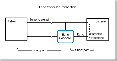
Fig.14
A typical echo canceller includes, apart from the adaptive FIR itself, a number of other modules that control the FIR adaptation process.
In Fig.15 a typical echo canceller adaptation process is showed. The noisy input signal from the talker generates the echo to be compensated. It can be seen that the difference between predicted and input echo (i.e. the residual echo) is diminishing (as a result of the FIR filter's adaptation).
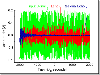
Fig.15