|
|
|
 |
General
The FIR algorithm calculates the convolution product vector y[] for an input data vector x[] and a weights data vector h[]. Each y[n] value of the output vector is calculated using the Convolution Product Kernel.
y[n]=CPK(x[],h[]);This results in a number of restrictions to be imposed on both the definition domains of the vectors and the numerical values in the vectors.
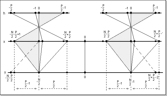
Fig. 2: Conditions for the definition domains so that an output
result can be uniquely calculated
Given the above formula, two basic variations of the FIR calculation problems will be considered:
- The problem asks for calculating the FIR output y[n] for n in
[-N/2, N/2-1], with a given wights function h() defined in [-P/2,
P/2-1]. In this case it can be seen from the CPK formula that it is
necessary and sufficient to have the input vector x[] defined in the
[-N/2-P/2, N/2+P/2-1]; the values of the input vector x[] outside the
[-N/2-P/2, N/2+P/2-1] are irrelevant.
The above condition is required for the general case of non-causal filters, i.e. when there is at least one coefficient h[k] non-zero for k<0.
For the special case of causal filters, i.e. h[k]=0 for every k in [-P/2,-1], it can be seen that the condition is relaxed to having the x[] vector defined in the [-N/2-P/2+1, N/2-1] interval.
Remark
An equivalent problem is obtained when one has x[] defined for a [-N/2, N/2-1] interval; in this case the output can be correctly calculated only for a sub-domain [-N/2+P/2-1, N/2-P/2]. Outside this interval one cannot correctly calculate the y[] output.
For the special case of causal filters, i.e. h[k]=0 for every k in [-P/2,-1], one can determine the output for the broader [-N/2+P/2-1, N/2-1] interval.
- The problem asks for a complete evaluation of the FIR output for
a given input vector x[]. This problem cannot be uniquely solved
without imposing restrictions on the input signal. The restrictions
consist in requiring that the input signal is an impulse, i.e. it has
to be Zero outside a specific domain (note that the y[] output will be
non-Zero in a larger domain than the domain in which the x[] input is
non-Zero). The non-causal and causal FIR cases will be treated
separately:
For the general non-causal filters:
Having x[] an impulse x[n]=0 for n outside [-N/2+P/2, N/2-P/2] results in:
y[n]=0 for n outside [-N/2, N/2-1], and
y[n]=CPK(x[],h[]) for n inside the [-N/2, N/2-1] domain.
Observation: The restriction x[n]=0 for n outside [-N/2+P/2, N/2-P/2-1] is included in the above.
For causal filters (h[k]=0 for k in [-P/2,-1]):
The restriction on the x[] input is relaxed to having x[] and impulse x[n]=0 for n outside the [-N/2, N/2-P/2]; the formula for calculating the y[] output remains the same.
Observation: The restriction x[n]=0 for n outside [-N/2, N/2-P/2-1] is included in the above.
Remark
An equivalent problem with the above is:
For the general non-causal filters,
Having x[] an impulse x[n]=0 for n outside [-N/2, N/2-1] results in:
y[n]=0 for n outside [-N/2-P/2, N/2+P/2-2], and
y[n]=CPK(x[],h[]) for n inside [-N/2-P/2, N/2+P/2-2].
Observation: The above y[n] formula also olds true for the [-N/2-P/2, N/2+P/2-1] domain.
For causal filters (h[k]=0 for k in [-P/2,-1]),
Having x[] an impulse x[n]=0 for n outside [-N/2, N/2-1] domain results in:
y[n]=0 for n outside [-N/2, N/2+P/2-2], and
y[n]=CPK(x[],h[]) for n inside [-N/2, N/2+P/2-2] domain.
Observation: The above y[n] formula also olds true for the [-N/2, N/2+P/2-1] domain.
Conditions for the numeric values involved in the FIR calculations
Given the CPK formula, it can be seen that the calculation of an
y[n] value involves repetitive additions of multiplication results.
Since the CDSP operates with fixed-point complex numbers that have
their real and imaginary parts in the [-1,1) domain it results that the
product's real and imaginary parts can overflow (in the (-2,2)
interval).
The first conditions imposed on the complex numeric values will be that
the modulus of any complex number (hereafter denoted by Abs()) has to
be smaller than one, i.e. Abs(Cx)<1. This will lead to having all
the complex products' modulus smaller than one.
Since there are P additions involved in the calculation of a y[n] value
it results that Abs(y[n]) < P. In order to have Abs(y[n])<1 the
condition imposed to the complex numbers vectors x[] and h[] will now
become Abs(x[i]*h[j])<1/P for any i,j.
This is enforced by the following general condition that guarantees the
lack of internal FIR calculations overflows: the maximum modulus of the
input samples times the maximum modulus of the weight factors must be
smaller than 1/P: Max(Abs(x[i])) * Max(Abs(h[j])) < 1/P for any i,j.
In this case the modulus of any output vector value will be smaller
than one, i.e. Abs(y[n])<1 for all n.
A number of sufficient conditions can now be derived from the above general condition:
- Abs(h[k])<1/P for any k, i.e. the modulus of each weight factor has to be smaller than 1/P
- Abs(x[n])<1/P for any n, i.e. the modulus of each input vector value has to be smaller than 1/P
- Abs(x[i])< Sqrt(1/P) and Abs(h[j])< Sqrt(1/P) for any i,j, i.e. both the modulus of each weight factor and the modulus of each input vector value have to be smaller than Sqrt(1/P)
Remark
The CDSP's arithmetic circuits are featured with overflow detection and
saturation mechanisms. This allows certain applications to use values
that generate overflows, if these applications are designed to
manipulate saturated results. In some circumstances this greatly
increases the dynamic range of the numbers involved in the fixed-point
calculations.
For example, in the case of a causal low-pass RC filter model, there
might be transitory output values that are greater than the input
(these can result due to the limitations of the discrete FIR model). If
a normalized (<1) amplitude rectangular impulse is fed in the FIR,
transient output values slightly bigger than the input (>1) can
result. However, given that the FIR is known to model a low-pass RC
filter, these values can safely be discarded and saturated without
impacting on the algorithm (see Fig.5d).
The FIR Implementation
The FIR components
The FIR module consists of the following user-accessible elements:
- the weight factors vector h[]; it has a programmable number of P elements
- an internal buffer vector t[] with the same size as h[]; this buffer stores the P input elements necessary to compute one y[n] output (using the CPK with the h[] vector)
- a function that defines P and loads the h[] vector
- a function that can be called to pre-fill the temporary buffer vector t[]
- a function that introduces one value into the temporary buffer vector t[]
- a function that extracts one FIR-calculated value; this function has two variants that are each optimized for non-causal and causal filters respectively
- a reset function that clears both the t[] and h[] vectors, and marks P as unassigned (set to -1).
The FIR usage
For the general non-causal FIR, given the fact that the computation of a y[n] output requires P input values to be known (i.e. x[n-P/2+1] to x[n+P/2]), it results that the first output sample can only be computed after introducing P input samples in the filter (this can be done via successive calls to the function that introduces one input sample at a time into the internal FIR temporary buffer t[]). These samples will represent P/2-1 samples "from the past", the "present" sample, and P/2 samples "from the future" in a time-domain interpretation (the non-causal filters output calculation requires samples both "before" and "after" the "present" moment). After introducing these P samples, one will be able to calculate a first FIR output. A new FIR output can further be calculated with each introduction of a new sample. Thus, the methodology of calculating the non-causal FIR filter output will consist of:
- introducing P/2-1 samples "from the past" (x[n0-P/2+1] to x[n0-1])
- introducing the "present" sample (x[n0])
- introducing P/2 samples "from the future" (x[n0+1] to x[n0+P/2])
- extracting the first FIR output value (y[n0])
- repetitively introducing a new input value representing an input "from the future" at time "present" +P/2 (x[n+P/2]) and calculating the "present" output (y[n]).
For the special case of the causal FIR, given the fact that the calculation of an output value y[n] only requires P/2 input values to be known (i.e x[n-P/2+1] to x[n]), it results that the first output sample can be computed after introducing P/2 input samples in the filter. These samples will represent P/2-1 samples "from the past", followed by the "present" sample in a time-domain representation (the causal filters output calculation only requires samples "from the past" and "present"). After introducing P/2 samples, one will be able to calculate the first FIR output. A new FIR output can further be calculated with each introduction of a new input sample. Thus, the methodology of calculating the causal FIR filter output will consist of:
- introducing P/2-1 samples "from the past" (x[n0-P/2+1] to x[n0-1])
- introducing the "present" sample (x[n0])
- extracting the first FIR output value (y[n0])
- repetitively introducing a new input value representing an input "from the present" (x[n]) and calculating the "present" output (y[n]).
In both the non-causal and causal cases, the condition for the output to be an impulse (to start with a zero value and end with a zero value) is that the first P and last P input values be zero.
Example 1
Ideal low-pass filter FIR approximation (non-causal)
Fig.4a shows the modulus of the transfer function of a non-causal ideal
low-pass filter in frequency domain (only the real part is non-zero,
while both the imaginary part and the phase characteristic of this
filter are flat zero on the whole frequency axis), and Fig.4b shows the
FIR coefficients for approximating this filter in the time domain (the
coefficients were calculated via an iFFT
transform; it can be seen that only the real part of the
coefficients results non-zero, the imaginary part is flat zero along
the whole time axis). Fig.4c and Fig.4d show a rectangular input signal
and its corresponding output from the FIR.
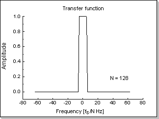 Fig.4a |
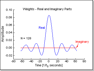 Fig.4b |
||
 Fig.4c |
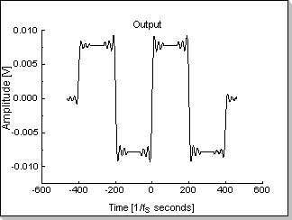 Fig.4d |
Remark 1
It can be seen in Fig. 4d that the output of the filter has some
transitory oscillations before the input signal's transitions;
this is as a result of the non-causality type of the filter.
Remark 2
The level of the input signal (Fig.4c) has been chosen smaller than
1/N, in this case x[n]<1/128. As previously described, this
guarantees the internal FIR calculations will not generate overflows.
Example 2
Low-pass RC filter FIR approximation (causal)
Fig.5a, 5b, and 5c show the transfer function of a causal RC low-pass
filter in frequency domain (modulus, phase, and the real and imaginary
parts), and Fig.5d shows the FIR coefficients (real and imaginary
parts) for approximating this filter in the time domain. Fig.5e and
Fig.5f show a rectangular input signal and its corresponding output
from the FIR.
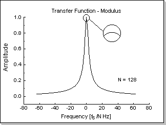 Fig.5a |
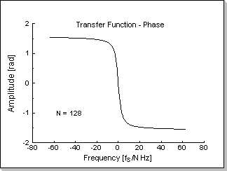 Fig.5b |
||
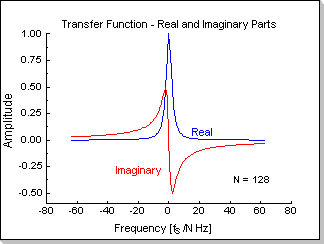 Fig.5c |
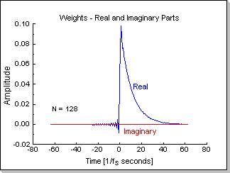 Fig.5d |
||
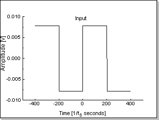 Fig.5e |
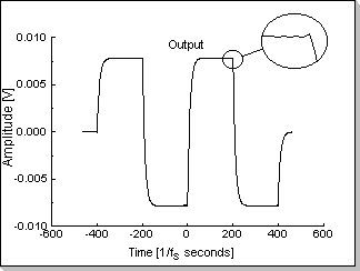 Fig.5f |
Remark 1
In this example the time-domain transfer function was obtained via an iFFT transform from the frequency-domain
transfer function. It can be seen in Fig.5d that the resulting
time-domain transfer function has small but non-zero values h[k]/=0 for
k<0. This is a result of the finite number of sampling points used
in the iFFT algorithm. As a result, in Fig.5f a small transitory value
bigger than the input value can be seen before the input signal's
transitions (i.e. the filter exhibits a perceptible non-causal
behavior).
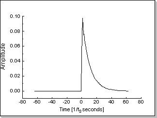 Fig.5g |
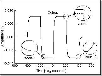 Fig.5h |
Fig.5g shows the time-domain transfer function obtained by "artificially" zero-ing the real part of all the FIR coefficients h[k] for k<0, and Fig.5h shows the resulting FIR response. It can be seen in Fig.5h, zoom1, that the filter no longer exhibits the non-causal behavior. However, because the coefficients were zero-ed without taking into consideration any of the side effects that this operation might cause, other types of distortions will appear; the most noticeable of these is the shift of the DC component of the output signal compared to the input signal (by setting h[k]=0 for k<0 the overall sum of the filter's coefficients is disturbed). This DC shift is represented in Fig.5h, zoom1, where the dashed line represents the input signal, and the continuous line represents the filter's output. The other two zooms in Fig.5h (zoom2, zoom3) show that parasitic transitory behavior has not been introduced in the filter response in any of the signal's singularity points.
Remark 2
The level of the input signal (Fig.5e) has been chosen smaller than
1/N, in this case x[n]<1/128. As previously described, this
guarantees the internal FIR calculations will not generate overflows.